Example of Split-Split Plot Design

Application Example

Experiments in agriculture want to study the effect of three factors, namely, Nitrogen fertilization (A), Management on crops (B) and Variety Type (C) on rice production yields (tons / ha).  Nitrogen factor is placed as the main plot, Management as a sub plot and varieties as sub-sub plots. 

Table 9      Rice Production Data (tons/ha)

Calculation by Hand:

Step 1: Calculate the Correction Factor

$$ CF=\frac{Y....^2}{rabc}=\frac{(502.221)^2}{3\times3\times3\times3}=3113.90$$ 

Step 2: Calculate the Sum of The Total Squares

$$\begin{matrix}SSTOT=\sum_{i,j,k,l}{Y_{ijkl}}^2-CF\\=(3.320)^2+(3.864)^2+...+(9.320)^2-3113.90\\=189.71\\\end{matrix}$$ 

Analysis of the Main Plot:

Main Total Plot Data (Block x Nitrogen)

Step 3: Calculate the Sum of The Main Plot Squares

$$\begin{matrix}SS(MP)=\sum_{i,l}\frac{{Y_{i..l}}^2}{bc}-CF=\frac{\sum_{i,l}{(a_ir_l)^2}}{bc}-CF\\=\frac{(49.331)^2+(49.598)^2+...+(63.601)^2}{3\times3}-3113.900\\=37.36\\\end{matrix}$$

Step 4: Calculate the Sum of Squares of Blocks

$$\begin{matrix}SSR=\sum_{l}\frac{{Y_{...l}}^2}{abc}-CF=\frac{\sum_{l}{(r_l)^2}}{abc}-CF\\=\frac{(166.583)^2+(171.433)^2+(164.205)^2}{3\times3\times3}-3113.90\\=1.005\\\end{matrix}$$

Step 5: Calculate the Sum of Squares of Factor A

$$\begin{matrix}SS(A)=\sum_{i}\frac{{Y_{i..}}^2}{rbc}-CF=\frac{\sum_{i}{(a_i)^2}}{rbc}-CF\\=\frac{(145.387)^2+(167.949)^2+(188.885)^2}{3\times3\times3}-3113.90\\=35.055\\\end{matrix}$$

Step 6: Calculate the Sum of Squares of Main Plot Errors (Ea)

$$\begin{matrix}SS(Ea)=\sum_{i,l}\frac{{Y_{i..l}}^2}{bc}-CF-SSB-SS(A)\\=\frac{\sum_{i,l}{(a_ir_l)^2}}{bc}-CF-SSB-SS(A)\\=SS(MP)\ -\ SSR\ -\ SS(A)\ \\=37.36-1.005-35.055\\=1.296\\\end{matrix}$$

Analysis of the Sub plot:

Total Sub plot Data: Block x Nitrogen x Management (RAB)

Total Nitrogen Factor x Management (AB) Data

Step 7: Calculate the Sum of Squares of Sub plots

$$\begin{matrix}SS(SP)=\sum_{i,j,l}\frac{{Y_{ij.l}}^2}{c}-CF\\=\frac{\sum_{i,j,l}{(a_ib_jr_l)^2}}{c}-CF\\=\frac{(14.776)^2+(14.522)^2+...+(23.629)^2}{3}-3113.900\\=63.07\\\end{matrix}$$

Step 8: Calculate the Sum of Squares of Factor B

$$\begin{matrix}SS(B)=\sum_{j}\frac{{Y_{.j..}}^2}{rac}-CF=\frac{\sum_{j}{(b_j)^2}}{rac}-CF\\=\frac{(152.086)^2+(163.598)^2+(186.537)^2}{3\times3\times3}-3113.90\\=22.785\\\end{matrix}$$

Step 9: Calculate the Sum of Squares of AB Interactions

$$\begin{matrix}SS(AB)=\sum_{i,j}\frac{{Y_{ij.}}^2}{rc}-CF-SS(A)-SS(B)\\=\frac{\sum_{i,j}{(a_ib_j)^2}}{rc}-CF-SS(A)-SS(B)\\=\frac{(43.864)^2+(46.575)^2+...+(69.069)^2}{3\times3}-3113.90-35.055-22.785\\=0.162\\\end{matrix}$$

Step 10: Calculate the Sum of Squared Sub plot Errors (Eb)

$$\begin{matrix}SS(Eb)=SS(SP)\ -\ SSR\ -\ SS(A)\ -\ SS(Ea)\ -\ SS(B)\ -\ SS(AB)\ \ \\=63.07-1.005-35.055-1.296-22.785-0.162\\=2.771\\\end{matrix}$$

Analysis of the Sub-sub plot:

Table of Nitrogen x Varieties (AC)

Management Table x Varieties (BC)

Nitrogen x Management x Variety (ABC) Table

Step 11: Calculate the Sum of Squares of Factor C

$$\begin{matrix}SS(C)=\sum_{k}\frac{{Y_{..k.}}^2}{rab}-CF\\=\frac{\sum_{k}{(c_k)^2}}{rab}-CF\\=\frac{(136.005)^2+(159.909)^2+(206.307)^2}{3\times3\times3}-3113.90\\=94.649\\\end{matrix}$$

Step 12: Calculate the Sum of Squares of AC Interactions

$$\begin{matrix}SS(AC)=\sum_{i,k}\frac{{Y_{i.k.}}^2}{rb}-CF-SS(A)-SS(C)\\=\frac{\sum_{i,k}{(a_ic_k)^2}}{rb}-CF-SS(A)-SS(C)\\=\frac{(40.618)^2+(42.873)^2+...+(77.074)^2}{3\times3}-3113.90-35.055-94.649\\=3.436\\\end{matrix}$$

Step 13: Calculate the Sum of Squares of BC Interactions

$$\begin{matrix}SS(BC)=\sum_{j,k}\frac{{Y_{.jk.}}^2}{ra}-CF-SS(B)-SS(C)\\=\frac{\sum_{j,k}{(b_jc_k)^2}}{ra}-CF-SS(B)-SS(C)\\=\frac{(40.065)^2+(43.878)^2+...+(77.388)^2}{3\times3}-3113.90-22.785-94.649\\=4.240\\\end{matrix}$$

Step 14: Calculate the Sum of Squares of ABC Interactions

$$\begin{matrix}SS(ABC)=\sum_{i,j,k}\frac{{Y_{ijk.}}^2}{r}-CF-SS(A)-SS(B)-SS(C)-\\SS(AB)-SS(AC)-SS(BC)\\=\frac{\sum_{i,j,k}{(a_ib_jc_k)^2}}{r}-CF-SS(A)-SS(B)-SS(C)-\\SS(AB)-SS(AC)-SS(BC)\\=\frac{(11.691)^2+(16.038)^2+...+(27.572)^2}{3}-3113.90-35.055-22.785-94.649-\\0.162-3.436-4.240\\=2.363\\\end{matrix}$$

Step 15: Calculate the Sum of Squares of Sub-sub plot Errors (Ec)

$$\begin{matrix}SS\left(Ec\right)=SSTOT-other\ SS\\=SSTOT-SSR-SS\left(A\right)-SS\left(Ea\right)-\\SS\left(B\right)-SS\left(AB\right)-SS\left(Eb\right)-\\SS\left(C\right)-SS\left(AC\right)-SS\left(BC\right)-SS\left(ABC\right)\\=189.709-1.005-35.055-1.296-\\22.785-0.162-2.771-\\94.649-3.436-4.240-2.363\\=21.947\\\end{matrix}$$

Step 16: Create an Analysis of variance Table with its F-Values table

Table 10.  Anova Table of Rice Yield

Calculate the coefficient of Variance:

$$\begin{matrix}CV(a)=\frac{\sqrt{MS(Ea)}}{\bar{Y}...}\times100\%=\frac{\sqrt{0.324}}{6.200}\times100\%\\=9.18\%\\\end{matrix}$$

$$\begin{matrix}CV(b)=\frac{\sqrt{MS(Eb)}}{\bar{Y}...}\times100\%=\frac{\sqrt{0.231}}{6.200}\times100\%\\=7.75\%\\\end{matrix}$$

$$\begin{matrix}CV(c)=\frac{\sqrt{MS(Ec)}}{\bar{Y}...}\times100\%=\frac{\sqrt{0.6096}}{6.200}\times100\%\\=12.59\%\\\end{matrix}$$

so: CV (a) = 9.18 %;  CV (b) = 7.75 %;  CV (c) = 12.59 %. 

The coefficient of Variance of the main plot > the sub-plot > the sub-sub plot.  But in the above case, it does not indicate the condition. If this happens frequently, you should discuss it with someone who is an expert in the field of statistics.

Step 17: Make a Conclusion

From the Analysis of variance Table, it does not appear that the effect of interaction is insignificant, both the interaction between the three factors (ABC interaction) and the interaction between two factors (AB, AC, BC), so that the examination of the effect of treatment is continued with its main effect.  The main (independent) effect of the three factors is significant, so it is necessary to carry out further investigation to determine the differences between the average levels of treatment.

Post Hoc

Based on the analysis of variance, the effect of interaction is not significant, while the three main effect are significant.  Further testing was conducted on the main-effect of these three factors.

Here are the post hoc test steps by using LSD:

Test criteria:

Compare the absolute value of the difference between the two averages that we will see the difference with the LSD value with the following test criteria:

 $$ if\ \ \left|\mu_i-\mu_j\right|\ \ \left\langle\ \ \begin{matrix}>LSD_{0.05}\ \mathbf{reject}\ H_0,\ two\ means\ are\ significantly\ different\\\le LSD_{0.05}\ \mathbf{accept}\ H_0,\ two\ means\ are\ not\ significantly\ different.\\\end{matrix}\right.$$

Comparison of Average Nitrogen Factors (A):

To compare the two main plot means (Nitrogen Factor), it is necessary to first determine the Standard Error (s_y) using the formula:

 $$s_{\bar{y}}=\sqrt{\frac{2MS(Ea)}{rbc}}$$

Specify the t-student value at the significant level of α =5% with error-degree of freedoms a = 4:

t_{(0.05/2; 4)} = 2.776

Calculate the LSD value:

$$\begin{matrix}LSD=t_{0.05/2;4}\cdot s_{\bar{Y}}\\=t_{0.05/2;4}\cdot\sqrt{\frac{2MS(Ea)}{rbc}}\\=2.776\times\sqrt{\frac{2(0.32399)}{3\times3\times3}}=2.776\times0.15492\\=0.430\ \ kg\\\end{matrix}$$

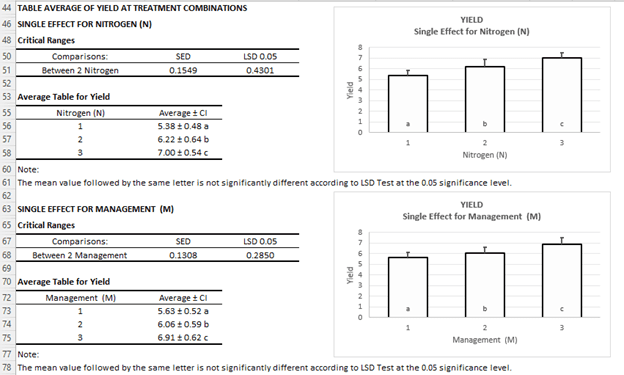
Compare the difference in the average treatment with the LSD value = 0.430 kg. State it differently if the average difference is greater than the LSD value.  The result is as follows: 

Comparison of Average Management Factors (B):

To compare two sub plot means (Management Factors), it is necessary to first determine the Standard Error (s_y) using the formula:

$$s_{\bar{y}}=\sqrt{\frac{2MS(Eb)}{rac}}$$

Specify the value of t-student at significant level α =5% with error-degree of freedoms b = 12:

t_{(0.05/2;  12)} = 2,179

Calculate the LSD value:

$$\begin{matrix}LSD=t_{0.05/2;12}\cdot s_{\bar{Y}}\\=t_{0.05/2;12}\cdot\sqrt{\frac{2MS(Eb)}{rac}}\\=2.179\times\sqrt{\frac{2(0.23094)}{3\times3\times3}}=2.179\times0.13079\\=0.285\ \ kg\\\end{matrix}$$

Compare the difference in the average treatment with the LSD value = 0.285 kg. State it differently if the average difference is greater than the LSD value. The result is as follows:

Comparison of Average Varietal Factors (C):

To compare two sub-sub plot means (Variety Factor), it is necessary to first determine the Standard Error (s_y) using the formula:

$$s_{\bar{y}}=\sqrt{\frac{2MS(Ec)}{rab}}$$

Specify the t-student value at a significant level of α =5% with error-degree of freedoms c = 36:

t_{(0.05/2;  36)} = 2,0281

Calculate the LSD value:

$$\begin{matrix}LSD=t_{0.05/2;36}\cdot s_{\bar{Y}}\\=t_{0.05/2;36}\cdot\sqrt{\frac{2MS(Ec)}{rab}}\\=2.0281\times\sqrt{\frac{2(0.60965)}{3\times3\times3}}=2.0281\times0.2125\\=0.4310\ \ kg\\\end{matrix}$$

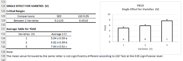
Compare the difference in the average treatment with the value of LSD = 0. 4310 kg. State it differently if the average difference is greater than the LSD value.  The result is as follows: 

Calculation by SmartstatXL Excel Add-In

Anova:

Post Hoc:

Interaction (Not Significant difference)

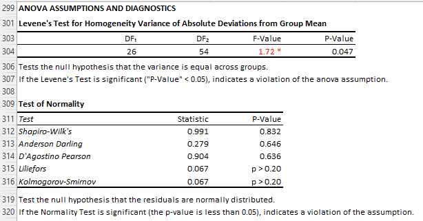
Anova Assumption: