Paired t-test

Hyphothesis

Assumption

1. The sample data contains paired elements
2. Samples taken randomly
3. Normally Distributed

Statistical Test

 $$ t=\frac{\bar{d}-\mu_d}{\frac{s_d}{\sqrt n}}$$

or if μ_d = 0, then:
 $$ t=\frac{\bar{d}}{\frac{s_d}{\sqrt n}}$$

Where is the degree of freedom (df) = n-1

d = difference between each individual/object in pairs

μ_d = the average value of the difference d of the population from the entire data pair, usually 0.

 $\bar{d}$ = the average value of d

s_d = standard deviation value from d

n = number of data pairs

Before performing data analysis with paired t-tests, we first test whether the two data spread normally or not. The test statistics used are the Lilliefors (Kolmogorov-Smirnov) normality test.

Normality test hypothesis:

• H₀ : Data spread normally
• H₁ : Data does not spread normally

On paired observations:

• Inter-sample or unit struggles were performed before the experiment began on the basis of expectation that if there was no effect of treatment then both groups gave the same response, and
• Source of variance from the outside is omitted, so the calculation of the value of the critique is based on the variance of differences between groups and not on the variance between individuals in each sample.

Example 1

The National Health Survey and Nutrition Testing, organized by the Department of Health and Public Services, examined the difference between self-reported and directly measured heights of some women between the ages of 12-16. Self-reported height and measured height data are presented in the Table below.

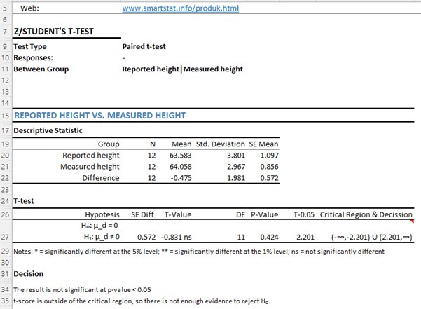
1. Is there enough evidence to support the allegation that there is a difference between the reported height and the measured height of women between the ages of 12-16? Use a significant level of 0.05.
2. Create a confidence interval with a 95% confidence level between the average difference in reported height and the measured height. 

Manual Calculation (Classical/Traditional Method)

1. Step 1: Claim: the alleged difference between the reported height and the measured height can be denoted by: μ_d ≠ 0, if the conjecture is false, then μ₁ = μ₂
2. Step 2: From the two equations above, the μ_d = 0 contains an element of equality, thus becoming a null hypothesis and alternative hypothesis (H₁) μ₁ ≠ μ₂.
3. H₀: μ_d = 0
4. H₁: μ_d ≠ 0
5. Significant level: α = 0.05
6. Determine the statistical test: the sample is randomly taken from the paired object so that the appropriate statistical test is a paired test.
7. Calculate t_stat and determine t_critical:
8.  $ t=\frac{\bar{d}-\mu_d}{\frac{s_d}{\sqrt n}}=\frac{-0.475-0}{\frac{1.981}{\sqrt{12}}}=-0.83$
9. Determine thet_critica with df = 12 and α = 0.05. From the t-student table obtained a critical t-value for a two-tailed test = ±2. 201 (sign due to Two-Tailed test±)
10. Because |t_stat| < |t_critical|= |-0.83| < | ±2.201|, then H₀ is welcome!
11. From the results of the t-test, it was concluded that at a significant level of 5%, there was not enough evidence to state a difference between the self-reported height and the height measured by the Department.

1. 95% confidence interval for average difference: Determine its Margin of Error Value (E)
   
   

 $$ E=t_{\alpha/2}\frac{s_d}{\sqrt n}=2.201.\frac{1.981}{\sqrt{12}}=1.258596$$

The confidence interval is calculated based on the following formula:

 $$\begin{matrix}\bar{d}-E<\mu_d<\bar{d}+E\\-0.475-1.259<\mu_d<-0.475+1.259\\-1.734<\mu_d<0.784\\\end{matrix}$$

That is, 95% of the average difference in the sample will lie in those intervals that in fact contain the average difference from the actual population.

Since the limit of the trust interval contains a value of 0, there is not enough evidence to support the allegation that there is a difference between the two heights.

Modern Methods:

The above method is a statistical test by traditional methods. Tests with modern methods use p-value in determining whether or not a statistical test is significant.

If: P-Value < Significant Level then the significant test or H₀ is rejected

If: P-Value > Significant Level then the non-significant test or H₀ is accepted

If the P-Value value < 0.01, then the test is very significant!

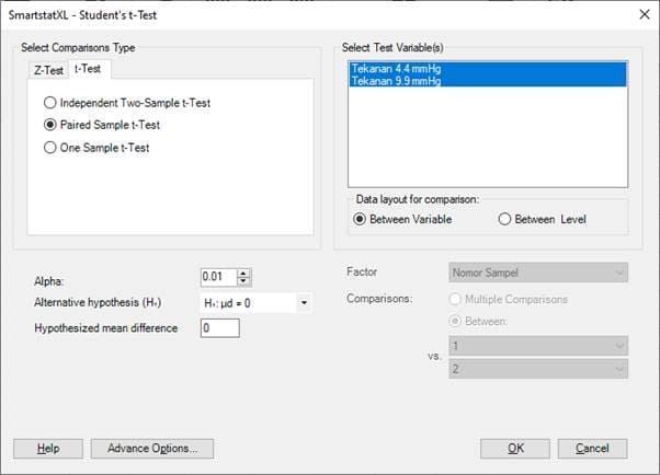
Calculations by using the SmartstatXL Excel Add-In

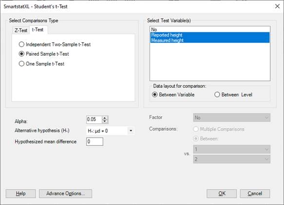
Analysis Results

Example 2

The effectiveness of a Tutoring in the face of a Test is assessed based on a comparison between the grades obtained by students before and after implementing the course. The score was obtained from 10 students who took the Entrance Preparatory Test Tutoring (based on data from the College Board and "An Analysis of the Impact of Commercial Test Preparation Courses on SAT Scores," by Sesnowitz, Bernhardt, and Knain, American Educational Research Journal, Vol. 19, No. 3.)

1. Is there enough evidence to conclude that Bimbel is effective in improving scores (test scores)? Test at a significant level of 0.05.
2. Determine the 95% confidence interval for the average difference between before and after following the Tutoring. Write down the statement and interpret the result.

Manual Calculation (Classical/Traditional Method)

1. Step 1: Claim: the allegation that after attending the Bimbel program can increase the score of the exam result can be denoted by: μ_d < 0, if the allegation is false, then μ₁ ≥ 0. (Why is the claim not symbolized μ_d > 0? If the value afterbimbel is greater, then the difference (d) must be negative, so it is symbolized by μ_d < 0 )
2. Step 2: From the two equations above, the μ_d ≥ 0 contains an element of equality, thus becoming a null hypothesis and alternative hypothesis(H₁) μ_d < 0.
3. H₀: μ_d = 0
4. H₁: μ_d < 0
5. Significant level: α = 0.05
6. Determine the statistical test: the sample is randomly taken from the paired object so that the appropriate statistical test is a paired test.
7. Calculate t_stat and determine t_critical:
8.  $ t=\frac{\bar{d}-\mu_d}{\frac{s_d}{\sqrt n}}=\frac{-11-0}{\frac{20.248}{\sqrt{10}}}=-1.718$
9. Determine t_critica with df = 9 and α = 0.05. From the t-student table obtained the t_critica value for the one tailed test = -1.833 (minus sign due to the left-tailed test)
10. Because |t_stat| < |t_critical|= |-1.718| < |-1.833|, then H₀ is accepted!
11. From the results of the t-test, it was concluded that at a significant level of 5%, there was not enough evidence to state that test preparation by taking a course (Bimbel) would be effective in improving test scores.

1. 95% confidence interval for the average difference:

Specify the Margin of Error Value (E)

 $$ E=t_{\alpha/2}\frac{s_d}{\sqrt n}=2.262\times\frac{20.248}{\sqrt{10}}=14.484$$

The confidence interval is calculated based on the following formula:

 $$\begin{matrix}\bar{d}-E<\mu_d<\bar{d}+E\\-11-14.484<\mu_d<-11+14.484\\-25.484<\mu_d<3.484\\\end{matrix}$$

That is, 95 % we believe that the average value of the difference from the actual population lies at an interval between 25.48 to 3.48.

Exercise 1

A researcher studied the influence of lighting on a Lucerne flower plant on different environmental conditions. Researchers took 10 plants that were fresh with flowers that were illuminated without hindrance at the top and hidden flowers at the bottom. Then, data on the number of seeds at each location were collected (Torrie, 1980). 

Hypothesis test there is no difference between the average population (H₀) and its counterpart (the flowers located at the top produce more seeds, H₁). Use a significant level of 0.05.

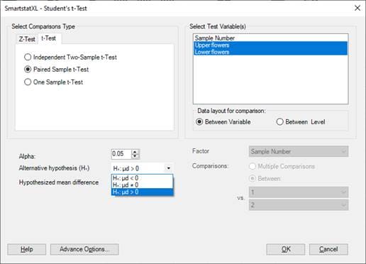
Calculations by using the SmartstatXL Excel Add-In:

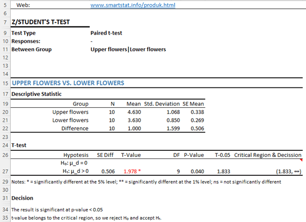
Analysis Results

Calculations using MINITAB Software v.19:

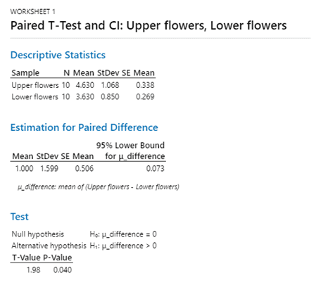
Interpretation:

Hypothesis:

3. H₀: μ_d = 0
4. H₁: μ_d > 0

Classic Method

t_stat = t_stat = T-Value = 1.98

t_critica = t_table = t_{(0.05.9) = 1,833} (obtained from the table value t-student)

Because |t_stat| > |t_critical| 1.98 > 1,833 then H0 is rejected!

That is to say: 95% of us believe that flowers located at the top produce more seeds compared to the flowers that are at the bottom of them.

Modern Methods:

Tests with modern methods use p-value in determining whether or not a statistical test is significant.

If: P-Value < Significant Level then the significant test or H₀ is rejected

If: P-Value > Significant Level then the non-significant test or H₀ is accepted

In the above case, P-Value = 0.040 which is a smaller value than the value of α = 0.05. This indicates that the test is significant or H₀ is rejected.

If the P-Value value < 0.01, then the test is very significant!

Exercise 2

As tested at a significant level of 0.01, is there a difference in the concentration of sugar in red clover nectar stored for 8 hours at two different pressures (4.4 mmHg and 9.9 mmHg)? Sugar concentration data are presented in the following Table.

Table of Sugar Content of red clover nectar (Torrie, 1980)

1. Hypothesis
2. H₀: μ₁ = μ₂
3. H₁: μ₁ ≠ μ₂
4. Significant level: α = 0.01

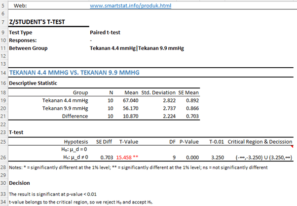
Calculations by using the SmartstatXL Excel Add-In:

Analysis Results

Calculations using MINITAB Software v.19:

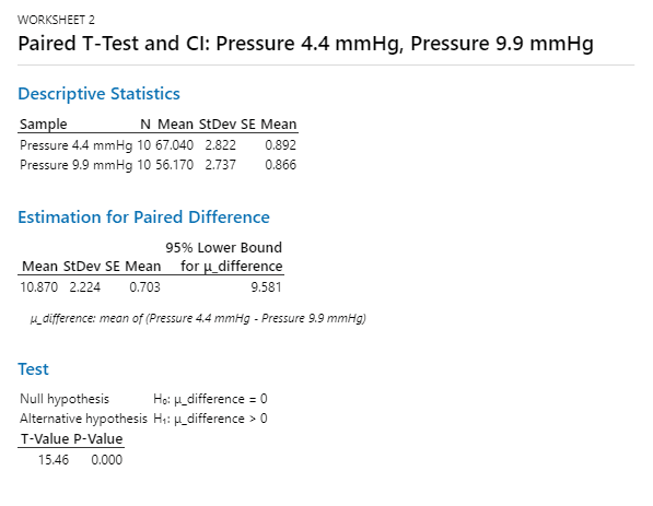
Interpretation:

Hypothesis:

1. H₀: μ_d = 0
2. H₁: μ_d ≠ 0

Classic Method

t_stat = t_stat = T-Value = 15.46

t_critica = t_table = t_(0.0 1.9) = 3,250 (Two-Tailed at significant level 1%)

Because |t_stat| > |t_critical| 15.46 > 3,250 then H₀ is rejected!

This shows that there is a very significant difference between the two pressures on sugar levels.

Modern Methods:

Tests with modern methods use p-value in determining whether or not a statistical test is significant.

If: P-Value < Significant Level then the significant test or H₀ is rejected

If: P-Value > Significant Level then the non-significant test or H₀ is accepted

In the above case, P-Value = 0.000 which is a smaller value than the value of α = 0.01. This indicates that the test is very significant or H₀ is rejected (P-Value value < 0.01)