How to Analyze Multinomial Regression

SmartstatXL offers a variety of regression analyses to model the relationship between independent and dependent variables. One such type of analysis that can be performed with SmartstatXL is Multinomial Logistic Regression.

Multinomial Logistic Regression is specifically designed for situations where the dependent variable is nominal with more than two levels or categories. Although similar to multiple linear regression in terms of predictive analysis, multinomial regression focuses on nominal dependent variables. Its primary objective is to explain the relationship between the dependent variable and one or more independent variables.

For example, if you want to predict someone's food preference based on several independent variables, the possible outcomes may include: Vegetarian, Non-Vegetarian, and Vegan.

Key features of multinomial (nominal) regression analysis with SmartstatXL:

1. Regression Diagnostics:
   • Outlier data information.
2. The ability to code outcomes in numerical form (0, 1) or text (Yes, No; Y, N; Success, Failure, etc.).
3. Event response adjustment for outcomes.
4. Outputs include:
   • Regression Equation.
   • Regression Statistics/Goodness of Fit: R², Cox-Snell R², Nagelkerke R², AIC, AICc, BIC, Log Likelihood.
   • Coefficient Estimation: Coefficient Value, Standard Error, Wald Stat, p-value, Upper/Lower, VIF.
   • Deviance Analysis Table.
   • Confusion Matrix (Classification Table and Metrics).

Case Example

Iris Dataset: Originally published in the UCI Machine Learning Repository.

Since 1936, the Iris dataset has been frequently used to test machine learning algorithms and visualizations. The Iris dataset is a classification dataset containing three classes, each with 50 instances, where each class refers to a type of iris plant. The three classes in the Iris dataset are: Setosa, Versicolor, Virginica. Each row in the table represents an iris flower, including its species and botanical dimensions, sepal length, sepal width, petal length, and petal width (in centimeters).

Author: R.A. Fisher (1936)

Source: UCI Machine Learning Repository

Steps for Multinomial Regression Analysis

1. Activate the worksheet (Sheet) that will be analyzed.
2. Place the cursor on the dataset (for creating a dataset, see Data Preparation methods).
3. If the active cell is not on the dataset, SmartstatXL will automatically attempt to identify the dataset.
4. Activate the SmartstatXL Tab
5. Click Menu Regression > Multinomial Regression.
   
6. SmartstatXL will display a dialog box to confirm if the dataset is correct (usually the dataset is automatically selected correctly).
   
7. If it's correct, click Next Button
8. Next, the Regression Analysis dialog box will appear: Select the Predictor Variables (Independent) and one or more Response Variables (Dependent).
   
9. Press the "Next" button
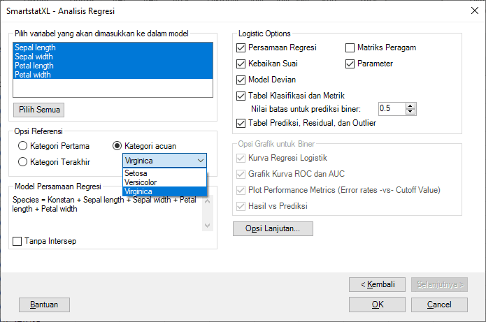
10. Select the regression output as shown in the following display (Suppose Reference=Virginica):
    
    The category used as the Reference can be the first category (SETOSA) or the last category (VIRGINICA). The reference category can also be directly selected from the outcome levels. In this example, suppose the Response Event is VIRGINICA.
11. Press the OK button to generate the output in the Output Sheet

Analysis Results

Analysis Information: type of regression used, regression method, response and predictors

In this Multinomial Regression analysis: "Species" is the response variable and the four predictors are "Sepal length", "Sepal width", "Petal length", and "Petal width".

Multinomial Regression Equation

The following are the multinomial regression equations:

1. Setosa:
   • Y=33.146+11.8539×Sepal length+13.3007×Sepal width−26.916×Petal length−37.9963×Petal width
   • For every one-unit increase in sepal length, the value of Y (likelihood of the species being Setosa) increases by 11.8539 units, assuming other variables remain constant.
   • For every one-unit increase in sepal width, the value of Y increases by 13.3007 units.
   • Conversely, for every one-unit increase in petal length, the value of Y decreases by 26.916 units.
   • And, for every one-unit increase in petal width, the value of Y decreases by 37.9963 units.
2. Versicolor:
   • Y=42.6378+2.4652×Sepal length+6.6809×Sepal width−9.4294×Petal length−18.2861×Petal width
   • For every one-unit increase in sepal length, the value of Y (likelihood of the species being Versicolor) increases by 2.4652 units, assuming other variables remain constant.
   • For every one-unit increase in sepal width, the value of Y increases by 6.6809 units.
   • Conversely, for every one-unit increase in petal length, the value of Y decreases by 9.4294 units.
   • And, for every one-unit increase in petal width, the value of Y decreases by 18.2861 units.
3. Model Evaluation Metrics:
   • R² is 0.964, which means that 96.4% of the variation in species can be explained by these four predictors. This indicates that our regression model fits the data very well.
   • The Chi-Squared value is 317.685 with a significance level (Sig) of 0.00. This indicates that our regression model is significant in predicting species based on the four given predictors.

In multinomial regression, we predict the logarithmic probabilities (log-odds) of a category against the reference category. In this case, it appears there are three categories (Setosa, Versicolor, and Virginica), but only two regression equations are given. This is because the third category (most likely Virginica) is considered the reference category, and its log-odds are zero (in logit scale).

To predict the outcome of an observation, follow these steps:

1. Calculate the log-odds for Setosa and Versicolor using the given regression equations.
2. Convert these log-odds to probabilities using the formula:
   • \[Probabilty = \frac{e^{log-odds}}{1 + e^{log-odds}}\]
3. The probability for Virginica can be calculated as:
   • \[Probability_{Virginica} = 1 - (Probability_{Setosa} + Probability_{Versicolor})\]
4. The category with the highest probability is considered the model's prediction for that observation.

Example Calculation:

Suppose we have an observation with the following characteristics:

• Sepal length = 5 cm
• Sepal width = 3.5 cm
• Petal length = 1.5 cm
• Petal width = 0.5 cm

Step 1: Calculate log-odds for Setosa and Versicolor

• Log-odds Setosa=33.146+11.8539(5)+13.3007(3.5)-26.916(1.5)-37.9963(0.5)= 79.5960
• Log-odds Versicolor=42.6378+2.4652(5)+6.6809(3.5)-9.4294(1.5)-18.2861(0.5)= 55.0599

Step 2: Convert log-odds to probabilities

\[Probability_{Setosa} = \frac{e^{Log-odds_{Setosa}}}{1 + e^{Log-odds_{Setosa}} + e^{Log-odds_{Versicolor}}} \approx 1\]

= 1

\[Probability_{Versicolor} = \frac{e^{Log-odds_{Versicolor}}}{1 + e^{Log-odds_{Setosa}} + e^{Log-odds_{Versicolor}}} \approx 0\]

= 0

Step 3: Calculate the probability for Virginica

\[Probability_{Virginica} = 1 - (Probability_{Setosa} + Probability_{Versicolor})\]

= 1 - (1 + 0)

= 0

Step 4: Determine the category with the highest probability

Based on calculations:

• The probability for Setosa is approximately 100%
• The probability for Versicolor is approximately 0%
• The probability for Virginica is also approximately 0%

Based on the obtained probabilities, our model will predict that this observation falls into the Setosa category because it has the highest probability.

In this example, our model is very confident that the given flower is Setosa, with a probability close to 100%. The probabilities for other categories are very low, close to zero.

Model Goodness of Fit

The following is an interpretation of the results for the goodness of fit or model accuracy in regression:

1. R² (Coefficient of Determination) = 0.9639:
   • The coefficient of determination (R²) measures how well the variation in the response variable is explained by the regression model. With an R² value of 0.9639, this means that 96.39% of the variation in species can be explained by our regression model. This is an indication of a very good fit between the model and the data.
2. Cox-Snell R² = 0.8797:
   • This is a goodness-of-fit measure adjusted for logistic regression. This value measures how well our model predicts the observed outcomes. A value approaching 1 indicates a good fit.
3. Nagelkerke R² = 0.9897:
   • Similar to Cox-Snell R², but this is a normalized version that has a more familiar range from 0 to 1. This value also indicates a very good fit between the model and the data.
4. AIC (Akaike Information Criterion) = 31.8985:
   • AIC measures the relative quality of a statistical model. A model with a lower AIC is considered better. This is important when comparing multiple models; the model with the lowest AIC is preferred.
5. AICc (Corrected Akaike Information Criterion) = 32.3152:
   • This is a version of AIC that has been corrected for sample size. In cases where the sample size is small and/or the number of predictors is high, AICc is preferred over AIC.
6. BIC (Bayesian Information Criterion) = 62.0049:
   • Like AIC, BIC is also used to compare the quality of models. However, BIC imposes a larger penalty for models with more parameters. Models with lower BIC are preferred.
7. Log Likelihood = -5.9493:
   • This is a measure of the likelihood that our model is the "correct" model. Higher values indicate a better model. Negative values are normal and can be interpreted as how far this value is from zero; the closer to zero, the better the model.

The above interpretation provides an overview of how well our regression model fits the given data and how well the model predicts the response based on the existing predictors.

Regression Coefficient Estimates

The following is an interpretation of the results for the estimated regression coefficients:

For the Setosa Species:

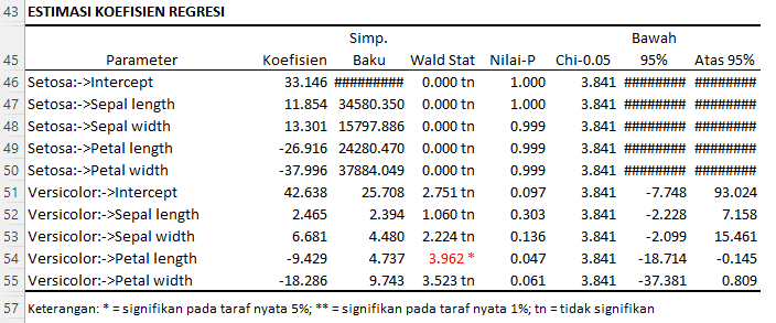
1. Intercept (Constant) = 33.146:
   • When all predictor variables are zero, the average value of the response (in the context of log-odds) for Setosa is 33.146. However, its very high standard deviation and Wald Stat value close to zero indicate that this estimate is unstable and possibly not significant.
2. Sepal Length:
   • For each one-unit increase in sepal length, the log-odds of Setosa increase by 11.854 units, assuming other variables remain constant. However, based on the Wald Stat and P-value, this coefficient is not significant at the 5% significance level.
3. Sepal Width:
   • For each one-unit increase in sepal width, the log-odds of Setosa increase by 13.301 units. This coefficient is also not significant at the 5% significance level.
4. Petal Length:
   • For each one-unit increase in petal length, the log-odds of Setosa decrease by 26.916 units. This coefficient is also not significant at the 5% significance level.
5. Petal Width:
   • For each one-unit increase in petal width, the log-odds of Setosa decrease by 37.996 units. This coefficient is also not significant at the 5% significance level.

For the Versicolor Species:

1. Intercept (Constant) = 42.638:
   • When all predictor variables are zero, the average value of the response (in the context of log-odds) for Versicolor is 42.638. This coefficient approaches significance at the 10% significance level.
2. Sepal Length:
   • For each one-unit increase in sepal length, the log-odds of Versicolor increase by 2.465 units. This coefficient is not significant at the 5% significance level.
3. Sepal Width:
   • For each one-unit increase in sepal width, the log-odds of Versicolor increase by 6.681 units. This coefficient is also not significant at the 5% significance level.
4. Petal Length:
   • For each one-unit increase in petal length, the log-odds of Versicolor decrease by 9.429 units. This coefficient is significant at the 5% significance level based on the Wald Stat and P-value.
5. Petal Width:
   • For each one-unit increase in petal width, the log-odds of Versicolor decrease by 18.286 units. This coefficient approaches significance at the 10% significance level.

Notes:

• Coefficients marked with the symbol (*) are significant at the 5% significance level. This means there is strong evidence that the coefficient is different from zero and has a real effect on the response.
• Coefficients without a symbol (tn) indicate that the coefficient is not significant at the 5% or 1% significance levels. This means there is no strong evidence that the coefficient is different from zero.

The above interpretation provides insights into the effect of each predictor on the response in the context of log-odds for each species.

Deviance/ Variance Analysis

Deviance analysis is used to evaluate how well our model predicts the observed data. Deviance is a measure of the lack of fit between the proposed model and the perfect model (which would predict the data perfectly).

1. Regression:
   • DF (Degrees of Freedom) = 9: This indicates the number of parameters estimated in the regression model, not including the constant.
   • Deviance = 317.685: This is the deviance resulting from our regression model. This deviance shows how far our model is from the perfect model.
   • P-Value = 0.000: This p-value indicates that our regression model is significant at the 1% significance level. In other words, there is strong evidence that our model predicts the response better than a model that only has a constant (without predictors).
   • Chi.05 = 16.919 and Chi.01 = 21.666: These are the critical values from the chi-square distribution at the 5% and 1% significance levels for 9 degrees of freedom. Since the deviance of our model (317.685) is much greater than both these critical values, it supports the conclusion that our model is significant.
2. Error:
   • DF (Degrees of Freedom) = 140: This indicates the number of observations minus the number of parameters estimated (including the constant).
   • Deviance = 11.8985: This is the residual deviance after considering the effects of the predictors in the model. It shows how far a model with only a constant (without predictors) is from the perfect model.
3. Total:
   • DF (Degrees of Freedom) = 149: Total degrees of freedom.
   • Deviance = 329.5837: Total deviance from the data.

Notes:

• Significant Deviance (**) at the 1% significance level indicates that our model has a good fit with the data and predicts the response better compared to a model that only has a constant.

The above interpretation provides insights into how well our regression model predicts the response variable (Species) based on the existing predictors.

Classification Table (Confusion Matrix)

Below is the interpretation of the results for the classification table and other classification metrics:

Classification Table

The classification table, also known as a confusion matrix, shows how our model classifies each case in the test or training data.

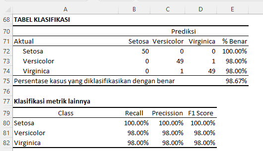
1. Setosa:
   • Of the 50 flowers that are actually Setosa, all 50 of them are correctly classified as Setosa by our model. This gives a classification accuracy rate of 100.00% for the Setosa species.
2. Versicolor:
   • Of the 50 flowers that are actually Versicolor, 49 are correctly classified as Versicolor, while 1 is misclassified as Virginica. This gives a classification accuracy rate of 98.00% for the Versicolor species.
3. Virginica:
   • Of the 50 flowers that are actually Virginica, 49 are correctly classified as Virginica, while 1 is misclassified as Versicolor. This gives a classification accuracy rate of 98.00% for the Virginica species.

Overall, our model correctly classifies 98.67% of all cases.

Other Classification Metrics

1. Recall (Sensitivity or TPR - True Positive Rate):
   • For Setosa, Versicolor, and Virginica, recall indicates the percentage of each actual species that is correctly classified by our model. A recall of 100.00% for Setosa means that all Setosa flowers are actually correctly classified.
2. Precision:
   • Precision indicates the percentage of our model's predictions that are actually accurate. For example, a precision of 100.00% for Setosa means that whenever our model predicts a flower as Setosa, the prediction is always correct.
3. F1 Score:
   • The F1 Score is the harmonic mean of recall and precision. This score provides an overall view of our model's performance in terms of the balance between recall and precision. A higher value indicates better performance.

From the above interpretation, we can see that our multinomial regression model performs exceptionally well in classifying the species of Iris flowers based on the existing predictors.

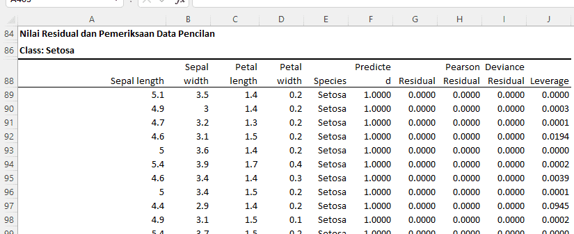
Residual Table

Class: Setosa

Class: Versicolor

Here is the interpretation for the residual analysis results and outlier data examination:

Class: Setosa

1. Residual: This indicates the difference between the actual observed values and the values predicted by the model. All observations have a residual of 0, meaning our model perfectly predicts the Setosa species for all these observations.
2. Pearson Residual: This is the residual normalized based on variance. All observations, except one, have Pearson residuals close to 0, indicating that our model's predictions align with the observations.
3. Deviance Residual: This provides a measure of how well our model predicts each individual observation. All observations have deviance residuals close to 0, indicating good predictions by our model.
4. Leverage: Measures how far the independent values of an observation are from the mean. Observations with high leverage (as indicated by "Extreme") have unusual or extreme predictor values.
5. Studentized Pearson Residual & Studentized Deviance Residual: These are residuals normalized based on the standard error. Large values of these metrics may indicate the presence of outliers.
6. Cook's Distance & DFITS: Both metrics provide a measure of an observation's influence on the model estimation. Observations with high Cook's Distance or DFITS values may have an unusual influence on the model.

Class: Versicolor

1. For this class, there are observations with "Outlier" as a diagnosis. This means our model has difficulty accurately predicting this observation, and the value predicted by the model is far from the actual observation.

Diagnostic:

• Outlier: Observations with large residuals are considered outliers. In this context, observations with "Outlier" as a diagnosis have significant residuals, indicating that our model does not predict these observations well.
• Extreme: Observations with high leverage values are considered extreme. In this context, observations with "Extreme" as a diagnosis have unusual or extreme predictor values.

From the above interpretation, we can see that although our model performs well for most observations, there are some observations that our model struggles to predict accurately.

Conclusion

Based on the analysis results, the following conclusions are drawn:

1. Regression Model: A multinomial regression model has been developed to predict the species of Iris flowers based on four predictors: sepal length, sepal width, petal length, and petal width. Two regression equations are provided, namely for Setosa and Versicolor, with Virginica considered as the reference category.
2. Model Performance: The model exhibits excellent fit with the data, with a coefficient of determination (R²) of 96.39%. This means that 96.39% of the variation in species can be explained by our regression model.
3. Model Goodness of Fit: Various metrics, such as Cox-Snell R², Nagelkerke R², AIC, BIC, and Log Likelihood, all confirm that our multinomial regression model fits well with the data.
4. Coefficient Estimates: Some coefficients are significant at the 5% or 1% level, indicating that certain predictors have a significant influence in predicting the species of Iris flowers. However, there are also some coefficients that are not significant, indicating that their effect may not be significant in the context of this model.
5. Classification: Our model successfully classifies 98.67% of all cases correctly, showing excellent effectiveness in classifying Iris species based on the given predictors.
6. Residuals and Outlier Diagnostics: Although our model performs well for most observations, there are some observations that our model struggles to predict accurately, as indicated by some significant residual values and 'Outlier' and 'Extreme' diagnoses.

Thus, based on the analysis conducted, the developed multinomial regression model shows excellent performance in predicting the species of Iris flowers based on their botanical characteristics. This model can be relied upon for future Iris species classification, taking into consideration the potential outliers or extreme observations that may affect predictions.

Writing in Scientific Reports

Multinomial Regression Analysis

Using multinomial regression analysis, a prediction model for Iris flower species was successfully developed. This model involves four predictor variables, namely sepal length, sepal width, petal length, and petal width. From the analysis, it was found that the model fits well with the data, as indicated by a coefficient of determination (R²) of 96.39%.

Model Performance

Based on the classification table, the model successfully classified 98.67% of all cases correctly. This indicates that the model is highly effective in classifying Iris flower species.

Outlier Diagnostics

Although the model shows good performance, there are some observations where the model struggles to predict accurately. This is marked by some significant residual values as well as observations labeled as 'Outlier' or 'Extreme'.

Conclusion

Based on the multinomial regression analysis conducted on the Iris flower dataset, it was found that four botanical characteristics, namely sepal length, sepal width, petal length, and petal width, have a significant influence in predicting Iris flower species. The developed model shows excellent fit with the data, with the ability to classify flower species with an accuracy of 98.67%. However, there are some observations where the model struggles to predict accurately, marked as outliers or extreme.