How to analyze the Completely Randomized Design - Single Factor Experiment

SmartstatXL is a specialized Excel Add-In designed to facilitate experimental data analysis. One of its applications is for the analysis of variance in a Completely Randomized Design (CRD) for a single factor. Currently, SmartstatXL only supports balanced designs. However, in addition to standard designs, SmartstatXL is also capable of managing data analysis with other mixed models.

The following is a list of menus and sub-menus related to single-factor CRD experiments available in SmartstatXL:

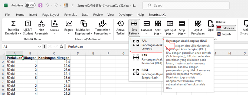
1. CRD: Pertains to single-factor CRD experiments where each observational unit is measured only once.
2. CRD: Sub-Sampling: Designed for multiple observations where sub-samples are drawn from a single observational unit. For illustration, in a single observational unit (e.g., Treatment 3Dok1, replicate 1), measurements are made on 10 plants.
3. CRD: Repeated Measure: Intended for multiple observations that are periodically measured from the same observational unit, such as every 14 days.
4. CRD: Multi-Location/Season/Year: This option is appropriate if the experiment is conducted in multiple locations, seasons, or years.
5. Kruskal Wallis Test (One Way Anova): If the assumptions for anova are not met, you can choose non-parametric analysis as an alternative for single-factor CRD.

Case Example

There is a study on the nitrogen content in milligrams from red clover plants injected with Rhizobium trifolii fungus, combined with a mixture of five strains of Rhizobium melitoti. There are six treatments; five of the treatments involve the transmission of R. trifolii and one strain of R. melitoti, while one treatment involves the combined transmission of all strains. The treatments are conducted in a greenhouse, where each treatment is applied to 5 pots of plants. A total of 30 pots with similar plants are provided. The injection of the six treatments is carried out randomly. The experiment uses a Completely Randomized Design (CRD).

Cited from:
Gaspersz, Vincent. 1991. Experimental Design Methods: For Agricultural Sciences, Engineering, and Biology. Bandung: Armico, 1991. p. 42.

Steps for Analysis of variancein CRD

1. Ensure that the worksheet (Sheet) you wish to analyze is active.
2. Place the cursor on the Dataset. (For information on creating a Dataset, please refer to the 'Data Preparation' guide).
3. If the active cell is not on the dataset, SmartstatXL will automatically detect and determine the appropriate dataset.
4. Activate the SmartstatXL Tab
5. Click on the Menu One Factor > Completely Randomized Design (CRD).
   
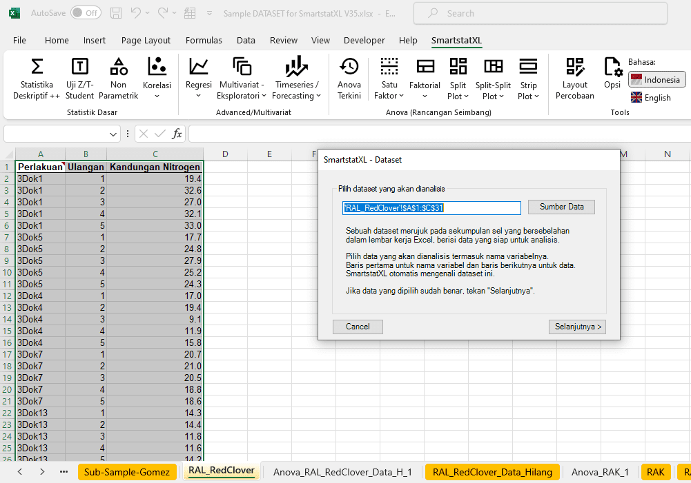
6. SmartstatXL will display a dialog box to confirm whether the Dataset is correct or not (usually, the cell address for the Dataset is automatically selected correctly).
   
7. After confirming the Dataset is correct, click Next Button
8. A dialog box titled Anova - Single Factor CRD will appear next.
   
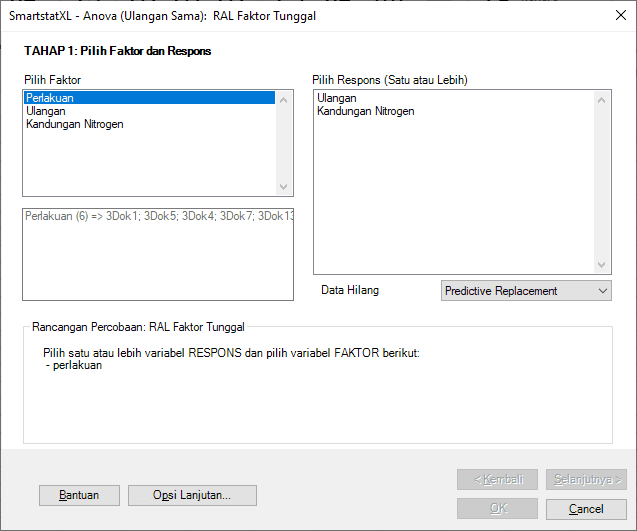
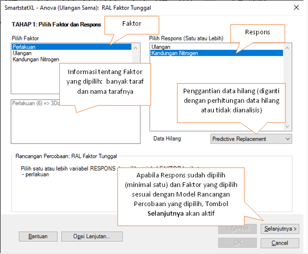
9. There are three stages in this dialog. In the first stage, select the Factor and at least one Response you wish to analyze.
10. When you select a Factor, SmartstatXL will provide additional information about the number of levels and their names. In CRD experiments, Replications are not included as a factor.
11. Details from the Anova STAGE 1 dialog box can be seen in the following image:
    
12. After confirming the Dataset is correct, click Next Button to proceed to Anova Stage-2 Dialog Box
13. A dialog box for the second stage will appear.
    
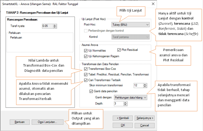
14. Adjust the settings based on your research methodology. In this example, the follow-up test used is the Tukey Test.
15. To set additional output and default values for subsequent outputs, click the "Advanced Options…" button.
16. The following is the display of the Advanced Options Dialog Box:
    
17. Once the settings are finalized, close the "Advanced Options…" dialog box.
18. Next, in the Anova Stage 2 Dialog Box, click the Next Button.
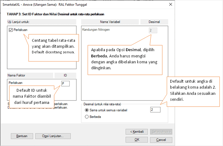
19. In the Anova Stage 3 Dialog Box, you will be asked to specify the average table, ID for each Factor, and rounding of average values. The details can be seen in the following image:
    
20. As a final step, click "OK"

Analysis Results

Analysis Information

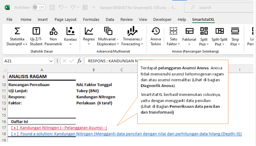
In a study concerning the nitrogen content in red clover plants injected with Rhizobium trifolii and a combination of five Rhizobium melitoti strains, analysis of variance (ANOVA) was conducted using a completely randomized design (CRD) with a single factor, which is the treatment. Six treatment levels were analyzed.

During the analysis, a violation of the ANOVA assumptions was found. The violation of these assumptions is critical as it can affect the validity of conclusions drawn from the analysis. To address this issue, SmartstatXL has found a solution by replacing outlier data using a value replacement method for missing data calculations. This method ensures that the data distribution meets the assumptions required by ANOVA, making the analysis more valid and reliable.

The use of the Tukey (BNJ) method as a post-hoc test indicates that after the ANOVA, comparisons between treatment groups will be made to identify which treatments significantly affect the nitrogen content.

Therefore, the subsequent ANOVA results will account for corrections made to outlier data, ensuring more accurate and valid interpretation.

Assumption Checks: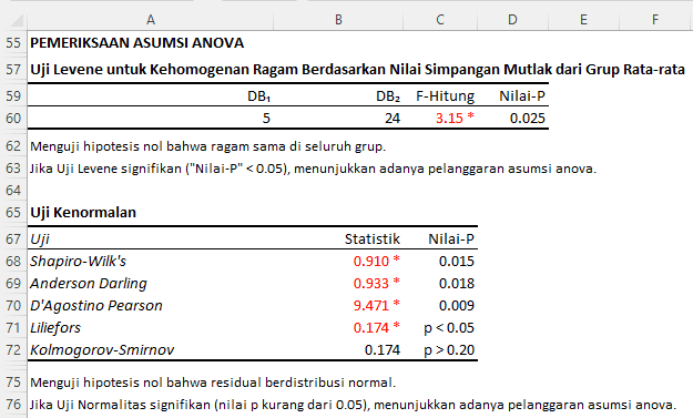

Interpretation and Discussion:

1. Levene's Test for Homogeneity of Variances: Levene's test was conducted to examine the assumption of homogeneity of variances across treatment groups. In this context, the calculated F-value for Levene's test was 3.15 with a p-value of 0.025. Given that this p-value is less than 0.05, it indicates that the assumption of homogeneity of variances has been violated. This means the variance of one or more treatment groups significantly differs from other treatment groups. Homogeneity of variances is an important assumption in ANOVA, so this violation needs attention and remediation before proceeding with the analysis.
2. Normality Test: The normal distribution of residuals is another important assumption in ANOVA. Based on the results provided:
   • Shapiro-Wilk's test shows a statistic value of 0.910 with a p-value of 0.015.
   • Anderson Darling has a statistic value of 0.933 with a p-value of 0.018.
   • D'Agostino Pearson shows a statistic value of 9.471 with a p-value of 0.009.
   • Liliefors test shows a statistic value of 0.174 with a p-value less than 0.05.
   • Whereas the Kolmogorov-Smirnov test shows a statistic value of 0.174 with a p-value greater than 0.20.

Out of the five normality tests conducted, four show a p-value less than 0.05, indicating a violation of the normality assumption. Only the Kolmogorov-Smirnov test indicates a normal distribution with a p-value greater than 0.05. However, considering the majority of tests indicate violation of the assumption, it can be concluded that the normal distribution assumption of the residuals has been violated.

Thus, the assumption checks reveal that the data used in this research violate two important assumptions in ANOVA: the homogeneity of variances and the normal distribution of residuals. Corrective action is needed before proceeding further with the analysis to ensure the validity and reliability of conclusions drawn. As a response to these violations, corrections have been made by replacing outlier data as previously mentioned.

Box-Cox Transformation: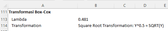

Data transformation is often used as an effort to meet statistical analysis assumptions, such as normality and homogeneity of variances in ANOVA. In the context of this research, a Box-Cox transformation is suggested with a lambda value of 0.481, leading to a square root transformation. However, despite the transformation, the violation of assumptions could not be resolved.

As an alternative, SmartstatXL tried another approach by correcting the outlier data. In some cases, outlier data can have a significant impact on data distribution and variance, thus removing or correcting them can help meet the required assumptions.

Solution:

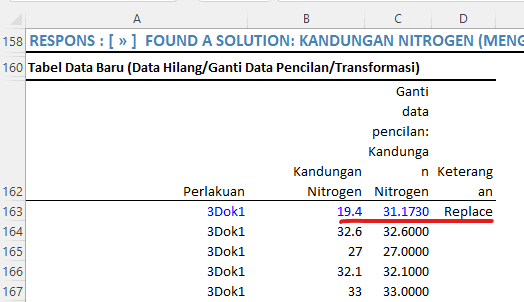
The analysis results indicate that this approach successfully mitigates the violation of assumptions. For instance, data with the treatment "3Dok1," originally having a nitrogen content of 19.4, was replaced with the value 31.1730 to address the outlier issue. Meanwhile, other data not considered as outliers have been retained at their original values.

By replacing outlier data using missing data calculations, the data distribution is now expected to satisfy the assumptions of analysis of variance (ANOVA), making subsequent analysis more valid and reliable.

It's important to note that the decision to replace outlier data should be carefully considered to ensure that it does not alter the fundamental characteristics of the data or the information that the study aims to convey. In this context, replacing outlier data is deemed an appropriate solution to maintain the integrity of statistical analysis without sacrificing important data insights.

Consequently, the upcoming ANOVA results will account for the corrections made to the outlier data, ensuring a more accurate and valid interpretation.

Variance Analysis

Interpretation and Discussion:

Analysis of variance (ANOVA) was performed to determine if there are significant differences in nitrogen content between treatment groups.

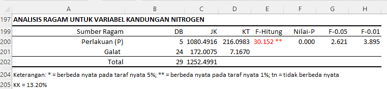
From the ANOVA table for the variable nitrogen content:

1. Treatment (P):
   • Degrees of Freedom (DF) for treatment is 5, indicating that there are six treatment groups (as DF = number of groups - 1).
   • Sum of Squares (SS) is 1080.4916 and Mean Square (MS) is 216.0983.
   • F-value for treatment is 30.152 with a p-value of 0.000. Given that this p-value is significantly less than 0.05 and 0.01, it can be concluded that there is a highly significant difference in nitrogen content between treatment groups. This is further confirmed by the double asterisk, which indicates that the difference is significant at the 1% level.
2. Error:
   • Degrees of Freedom (DF) for error is 24.
   • Sum of Squares (SS) is 172.0075 and Mean Square (MS) is 7.1670. This provides an insight into the variability in the data not explained by the treatment.
3. Total:
   • Sum of Squares (SS) total is 1252.4991.

In addition, it is provided that the Coefficient of Variation (CV) is 13.20%. This indicates that approximately 13.20% of the data variability is explained by the treatment.

Therefore, it can be concluded that the treatment has a significant impact on the nitrogen content. In other words, at least two treatment groups have significantly different average nitrogen contents. Further tests can be conducted to determine which treatment groups differ from each other.

Post Hoc Test

The appearance of tables and graphs can be adjusted via Advanced Options (refer back to step 15 of the Steps of Analysis of Variance).

Interpretation and Discussion:

A Tukey post hoc test (HSD) was conducted to identify specific differences between treatment groups based on average nitrogen content.

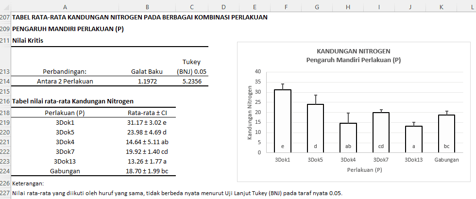
Critical Value:

The table provides information that the Standard Error between two treatments is 1.1972. The critical value for the Tukey (HSD) test at a 0.05 significance level is 5.2356. This means that the average difference between two treatments must be greater than 5.2356 to be considered significant at the 5% level.

Table of Average Nitrogen Content:

• The "3Dok1" treatment has an average nitrogen content of 31.17 with a confidence interval of ± 3.02 and is coded as "e".
• The "3Dok5" treatment has an average of 23.98 with a confidence interval of ± 4.69 and is coded as "d".
• ...and so on

Based on the letter codes, we can interpret the comparisons between treatments as follows:

• The "3Dok1" treatment significantly differs from all other treatments.
• The "3Dok5" treatment significantly differs from "3Dok4", "3Dok7", "3Dok13", and "Combined", but not from "3Dok7".
• The "3Dok4" treatment does not significantly differ from "3Dok13" and "Combined".
• The "3Dok7" treatment does not significantly differ from "3Dok5" and "Combined".
• The "3Dok13" treatment does not significantly differ from "3Dok4".
• The "Combined" treatment does not significantly differ from "3Dok4" and "3Dok7".

Therefore, the Tukey post hoc test (HSD) has identified which treatments have significantly different average nitrogen contents from others at a 0.05 significance level. This information is crucial for providing specific recommendations or conclusions based on the research findings.

Examination of ANOVA Assumptions

Formal Approach (Statistical Tests)

Interpretation and Discussion:

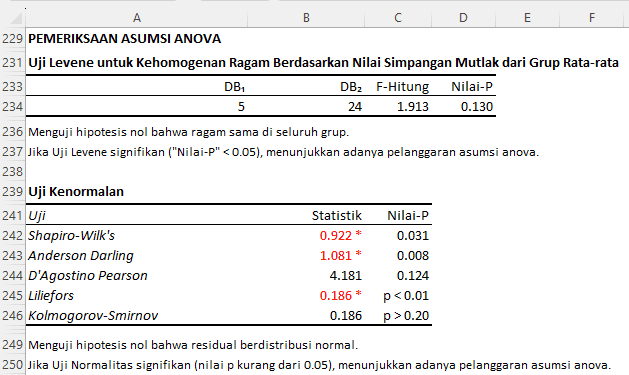
1. Levene's Test for Homogeneity of Variances: Levene's test was conducted to examine the assumption of homogeneity of variances across treatment groups. In this context, the F-value for Levene's test is 1.913 with a p-value of 0.130. Because this p-value is greater than 0.05, there is insufficient evidence to reject the null hypothesis. Therefore, the assumption of homogeneity of variances is considered met. The variance of each treatment group is considered equal.
2. Normality Test: The normal distribution of the residuals is another critical assumption in the analysis of variance. Based on the provided results:
   1. The Shapiro-Wilk's test shows a statistical value of 0.922 with a p-value of 0.031.
   2. The Anderson-Darling test has a statistical value of 1.081 with a p-value of 0.008.
   3. The D'Agostino Pearson test shows a statistical value of 4.181 with a p-value of 0.124.
   4. The Liliefors test shows a statistical value of 0.186 with a p-value less than 0.01.
   5. Whereas, the Kolmogorov-Smirnov test shows a statistical value of 0.186 with a p-value greater than 0.20.

Out of the five normality tests conducted, three of them indicated that the p-value is less than 0.05, suggesting a violation of the normality assumption. Only the D'Agostino Pearson and Kolmogorov-Smirnov tests indicated a normal distribution with a p-value greater than 0.05. However, considering that the majority of tests point to a violation of the assumption, it can be concluded that the assumption of normal distribution of residuals has been violated.

In conclusion, based on the assumption checks that have been performed, the data used in this study meet the assumption of homogeneity of variances but violate the assumption of normal distribution of residuals; only two tests assert that the residual values are normally distributed. Despite this, violations of the normality assumption can often be tolerated, especially if the sample size is sufficiently large. Nevertheless, it should be remembered that violation of assumptions can affect the validity of conclusions drawn from the analysis of variance. Therefore, it is important to consider alternative analytical methods or apply corrections to the data to ensure the normality assumption is met before proceeding with further analysis.

Note: You can change the minimum transformation score to 16 (Default is 12=one or two normality tests are sufficient). We will demonstrate this at the end.

Visual Approach (Plotting Graphs)

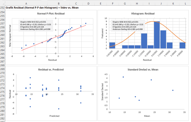
In addition to formal tests, assumption checks can also be performed visually using the included residual plots. These checks can be conducted using Normal Probability Plot (Normal P-Plot), Histogram, Residual vs. Predicted Plot, and Standard Deviation vs. Mean Plot.

Normal P-Plot for Residuals:

The Normal P-Plot is used to examine whether the data (in this case, residuals) follow a normal distribution. Ideally, the points on this plot should follow a straight diagonal line. If the points deviate from the diagonal line, this may indicate deviations from normality.

From the graph visualization:

• Most points appear to follow the diagonal line, suggesting that most residuals follow a normal distribution.
• However, there are some points, particularly at the left and right tails of the graph, that deviate from the diagonal line. This indicates the presence of some residuals that do not follow a normal distribution and could be considered outliers.

Therefore, based on the Normal P-Plot visualization, residuals largely follow a normal distribution with a few exceptions at extreme values. These deviations may affect the analysis results and the model's validity. Therefore, it is crucial to consider appropriate measures, such as replacing outlier data or transforming the data, to obtain a more reliable model.

Histogram for Residuals:

The histogram graph is used to visualize data distribution. In this context, we use the histogram to examine the distribution of residuals. The histogram should show a distribution that approximates a bell shape (normal distribution). Deviations from this shape (e.g., skewed or long-tailed distribution) may indicate violations of the normality assumption.

From the histogram visualization:

• The distribution shape appears to approximate a bell shape, indicating that the distribution of residuals tends to be normal.
• There is no significant skewness or clear asymmetry trend in the histogram, suggesting that the distribution of residuals is generally symmetrical.
• Although there are some peaks, there are no clear modes or very high frequencies at specific points, indicating that no group of residuals is overly dominant.

Therefore, based on the histogram visualization, the residual distribution seems to approximate a normal distribution. This indicates that the normality assumption for residuals, one of the key assumptions in variance analysis, tends to be met. This adds confidence to the validity and reliability of the analysis of variancemodel being used.

Residual vs. Predicted:

Homoscedasticity:

• If residuals are randomly scattered around a horizontal line at value 0 and show no particular pattern (e.g., funnel shape or U-shape), then the assumption of homogeneity is considered to be met. If there is a pattern, such as a funnel shape, this indicates heteroscedasticity, meaning that residual variability changes with the predicted values.
• Points appear to be randomly scattered around a horizontal line at value 0 and show no particular pattern, indicating that data variability is consistent across the range of predicted values. This suggests that the homoscedasticity assumption tends to be met.

Independence:

• If residuals are randomly scattered and show no pattern of autocorrelation (e.g., wave-shaped or cyclical patterns), then the independence assumption is considered to be met.
• There is no clear wave-shaped or cyclical pattern, indicating that residuals are independent and not autocorrelated.

Therefore, based on the visualization of the predicted vs. residual graph, the assumptions of homoscedasticity and independence for residuals appear to have been met. This suggests that the analysis of variancemodel has met two important assumptions and the results from this model can be considered reliable.

Standard Deviation vs. Mean Graph

The Standard Deviation vs. Mean graph is used to examine the homogeneity assumption in data in a different way from the Predicted vs. Residual graph.

In the Standard Deviation vs. Mean graph:

• The horizontal axis (X-axis) represents the mean value of each group or category.
• The vertical axis (Y-axis) represents the standard deviation of each group or category.

How to read the Standard Deviation vs. Mean graph is as follows:

Homoscedasticity: If points on the graph do not show a clear correlation pattern (e.g., straight line ascending or descending), then the homoscedasticity assumption is considered to be met. Conversely, if there is a clear positive or negative correlation between the mean and standard deviation, this indicates heteroscedasticity, meaning that data variability changes with the mean value.

From the visualization:

• Points appear to be scattered without a clear correlation pattern between standard deviation and mean. This indicates that data variability (standard deviation) is consistent across the range of mean values.

Therefore, based on the visualization of the Standard Deviation vs. Mean graph, the homoscedasticity assumption appears to have been met. This suggests that data variability is consistent across the range of mean values, and further analysis on this data is considered valid.

Residual Analysis

Interpretation and Discussion:

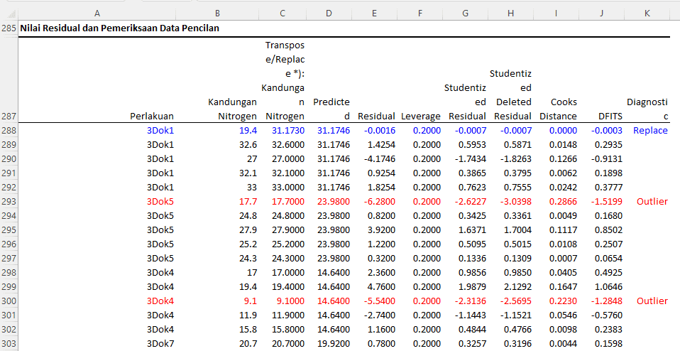
In the table displayed, a residual analysis is conducted to verify the validity of the analysis of variance model and to identify the presence of potential outliers or extreme values.

From the table, several key points to note include:

1. Residual: Represents the difference between the actual observed values and the values predicted by the model. A large residual indicates that the model fails to accurately predict the data.
2. Leverage: Measures how far the predictor value (X) is from the mean of the predictor values. High leverage values indicate that the data has extreme predictor values.
3. Studentized Residual: A standardized residual used for identifying outliers.
4. Studentized Deleted Residual: Similar to the studentized residual but calculated by removing certain observations from the model.
5. Cook's Distance: Measures the influence of the deletion of a particular observation on all coefficients of the model. A high value indicates that the observation significantly influences the model.
6. DFITS: Measures how far the prediction for a particular observation changes when that observation is removed from the analysis. A high DFITS value indicates that the observation is different from the other observations.

For illustration:

• The first observation under the treatment "3Dok1" with a nitrogen content of 19.4 (changed to 31.1730) has a very small residual (-0.0016) and is not considered an outlier.
• An observation under the treatment "3Dok5" with a nitrogen content of 17.7 has a large residual (-6.2800) and is identified as an outlier.

Thus, based on the residual analysis, it can be concluded that there are several observations considered as outliers or having extreme values. These observations may impact the outcome of the analysis and the model's validity. Therefore, it is crucial to consider appropriate measures, such as replacing outlier data with missing data formulas or transforming the data, to ensure more accurate and reliable analysis results.

Transformation: Transformation Score

Based on assumption checks, the variance of the residual data is homogeneous. However, out of the five normality tests, only two indicate that the residual values are normally distributed. If it is required for the residual values to be normally distributed in all normality tests, you can change the minimum transformation score to 16 (Default is 12= sufficient if one or two normality tests are met).

If the minimum transformation score is raised (for example, to 16) so that all normality tests are met: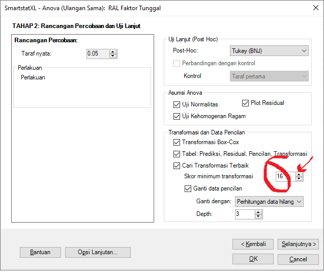

Here is the new data table after the transformation score is increased to 16. Some data considered outliers are replaced with new data.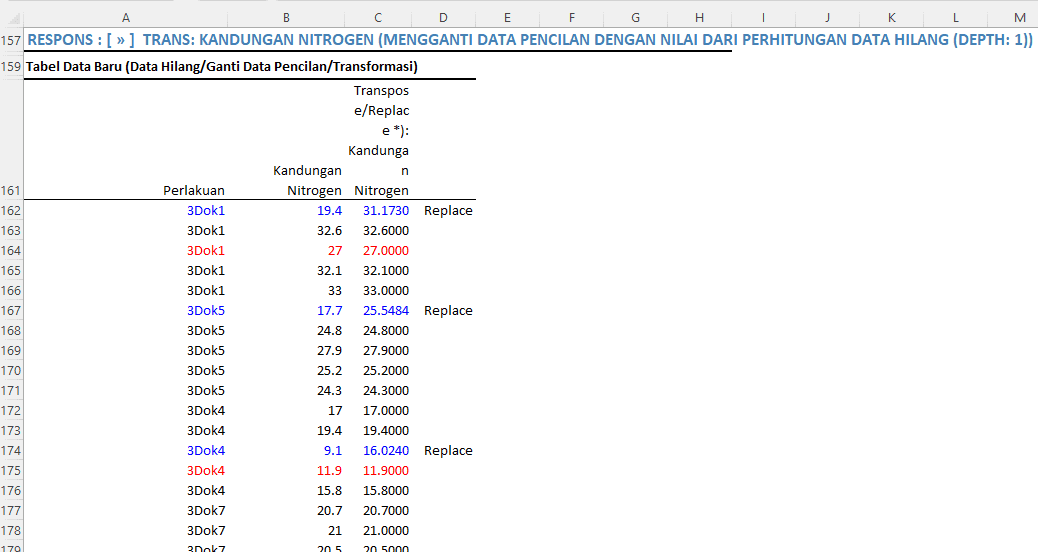

Results of Homogeneity and Normality Tests: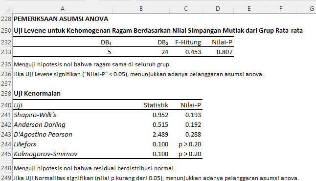

After raising the transformation score to 16, the assumptions of variance homogeneity and normality are met. All normality tests indicate that the residual data is normally distributed.

Average Values Table after replacing some data with missing data calculations: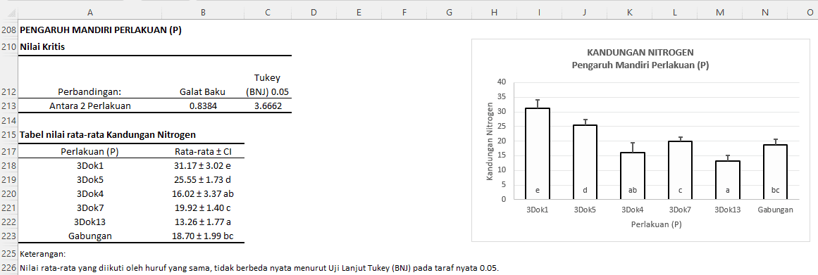

Conclusion

1. Analysis of varianceand Assumptions: In the study on nitrogen content in red clover plants, an analysis of variance (ANOVA) is employed using a Completely Randomized Design (CRD) to assess differences between treatments. Initial assumptions for the analysis of variance were violated, particularly in terms of variance homogeneity and data normality. However, solutions were found by replacing outlier data, allowing for the analysis of variance to proceed.
2. Analysis of varianceResults: Based on the analysis of variance, there is a significant difference between treatments at a 1% significance level. This indicates that the treatments have an effect on the nitrogen content in the plants.
3. Post Hoc Test: The follow-up Tukey test shows specific differences between treatment combinations. For instance, the treatment "3Dok1" shows a significant difference compared to all other treatments.
4. Examination of Homogeneity and Normality Assumptions: Through the predicted vs. residual graphs and histograms for residual data, the assumptions of homogeneity and normality of residuals appear to be met. This adds confidence to the analysis of varianceresults.
5. Standard Deviation vs. Mean Graph: This graph is used to check the assumption of homoscedasticity of the data, with results indicating no correlation between the mean and standard deviation, reaffirming that the homoscedasticity assumption is met.

Therefore, despite initial hurdles in meeting the assumptions of variance analysis, appropriate solutions have allowed the analysis to proceed and produce valid and reliable findings. The treatments administered to the red clover plants have an effect on the nitrogen content, with some treatment combinations showing significant differences.