How to Conduct Discriminant Analysis

Discriminant analysis is a statistical technique used to distinguish or predict groups based on the differences among those groups. This technique is very useful in various fields, such as psychology, medical, market, agricultural research, and others, where we need to understand classification or groups.

Discriminant analysis works by developing one or more discriminant functions that help distinguish between different groups based on a combination of selected variables. The discriminant function can be considered as a line or surface that separates groups. The value of the discriminant function can be used to predict which group a particular case belongs to.

There are two main types of discriminant analysis:

1. Linear Discriminant Analysis: Used when the independent variables are metric and assumed to have a normal distribution and equal variance across all groups.
2. Quadratic Discriminant Analysis: Used when the independent variables are metric and assumed to have a normal distribution, but the variance may differ among groups.

The steps in discriminant analysis include:

1. Identifying the independent and dependent variables.
2. Checking the assumptions of discriminant analysis (e.g., normality, equal variances, correlation among independent variables).
3. Creating the discriminant function.
4. Interpreting the discriminant function.
5. Testing the validity of the discriminant model.
6. Using the discriminant function to predict groups.

Essentially, discriminant analysis is a way to understand and utilize differences between groups in order to make effective predictions or classifications.

Case Example

Here is an example case of Linear Discriminant Analysis on Soil Texture Data and Its Relationship with Yield, Water, and Herbicide. This study focuses on linear discriminant analysis of soil texture data and its relationship with yield, water, and herbicide. The data consists of four types of soil textures: loam, sandy, salty, and clay. Each soil texture is measured based on three variables, namely yield, water, and herbicide.

Cited from:
https://real-statistics.com/free-download/real-statistics-examples-workbook/

Description:

• Texture: Type of soil texture (e.g., loam, sandy, salty, clay).
• Yield: Output (such as harvest yield in kilograms per hectare or maximum possible percentage).
• Water: Water content in the soil (e.g., in percentage).
• Herbicide: Use of herbicides (e.g., in kg/hectare or number of applications).

Discriminant analysis is a statistical technique used to distinguish or predict categorical variables based on a set of predictor variables. In this case, the discriminant analysis method can be used to predict the type of soil texture based on predictor variables: yield, water content (water), and herbicide use (herbicide).

Here are some things we can learn from discriminant analysis:

1. Discriminant Function: This analysis will generate a discriminant function for each group (in this case, each type of soil texture: loam, sandy, salty, and clay). This function will show the combination of predictor variables (yield, water, herbicide) that are most effective in distinguishing between types of soil textures.
2. Group Separation: You will be able to see how far each type of soil texture can be separated based on predictor variables. For example, if the yield and water content are very different for loam compared to other soil types, the discriminant analysis will show this.
3. Prediction: Once the discriminant function has been determined, you can use it to predict the type of soil texture based on yield, water, and herbicide. This can be very useful if you have new data and want to predict the type of soil texture without having to directly test the soil.
4. Importance of Predictor Variables: Discriminant analysis can also tell you how far each predictor variable (yield, water, herbicide) contributes in distinguishing between types of soil textures. For example, if yield is the most important factor in distinguishing soil texture types, the discriminant analysis will show this.

Remember that discriminant analysis assumes that your data meet several assumptions, including normality, homoscedasticity, and independence of observations. If these assumptions are not met, the results of the analysis may not be accurate or can be misleading.

Steps for Discriminant Analysis:

1. Activate the worksheet (Sheet) to be analyzed.
2. Place the cursor on the Dataset (to create a Dataset, see the Data Preparation method).
3. If the active cell (Active Cell) is not on the Dataset, SmartstatXL will automatically try to determine the Dataset automatically.
4. Activate the SmartstatXL Tab.
5. Click Menu Multivariate > Discriminant Analysis.
   
6. SmartstatXL will display a dialog box to confirm whether the Dataset is correct or not (usually the cell address of the Dataset is automatically selected correctly).
   
7. If it's correct, Click the Next Button.
8. Next, the Discriminant Analysis Dialog Box will appear:
   
9. Select the Predictor Variable (Independent) and one or more Group Variables (Dependent). In this case, we determine:
   • Predictor: Yield, Water, Herbicide
   • Group/Cluster: Texture
   • Discriminant Function: Linear Discriminant Analysis
   • Prior: All groups are the same

   Details can be seen in the following dialog box display:
   

10. Press the "Next" button.
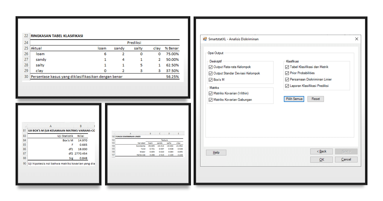
11. Select Discriminant Analysis output as shown in the following display by pressing the Select All button:
    
12. Press the OK button to create its output in the Output Sheet.

Analysis Results

Analysis Information and Classification Table.

The above table is the classification table or confusion matrix from the discriminant analysis. It shows how accurate the discriminant model is in classifying data based on predictions compared to actual values.

Here is the interpretation of the table:

1. Loam: From 8 actual observations with "loam" soil texture, the model correctly predicted 6 as "loam" and the model incorrectly predicted 2 as "sandy". The classification accuracy for "loam" is 75.00% (6 out of 8 observations were correctly classified).
2. Sandy: From 8 actual observations with "sandy" soil texture, the model correctly predicted 4 of them as "sandy". The model incorrectly predicted 1 observation as "loam", 1 observation as "salty", and 2 observations as "clay". The classification accuracy for "sandy" is 50.00% (4 out of 8 observations were correctly classified).
3. Salty: From 8 actual observations with "salty" soil texture, the model correctly predicted 5 of them as "salty". The model incorrectly predicted 1 observation as "loam", 1 observation as "sandy", and 1 observation as "clay". The classification accuracy for "salty" is 62.50% (5 out of 8 observations were correctly classified).
4. Clay: From 8 actual observations with "clay" soil texture, the model correctly predicted 3 of them as "clay". The model incorrectly predicted 2 observations as "sandy" and 3 observations as "salty". The classification accuracy for "clay" is 37.50% (3 out of 8 observations were correctly classified).

Overall, the model correctly classified 56.25% of all cases. This means that more than half of the model's predictions are correct, but there is room for improvement.

Other Classification Metrics

Other known classification metrics are recall (sensitivity or true positive rate), precision (precision or positive predictive value), and F1 score. Here are the interpretations:

Loam:

• Recall of 75.00% means that of all actual "loam" observations, the model correctly identified 75.00%.
• Precision of 75.00% means that of all observations predicted as "loam", 75.00% of them were indeed "loam".
• F1 Score of 75.00% is the harmonic mean of recall and precision. A high value indicates that the model has both good recall and precision for the "loam" class.

Sandy:

• Recall of 50.00% means that of all actual "sandy" observations, the model correctly identified 50.00% of them.
• Precision of 44.44% means that of all observations predicted as "sandy", 44.44% of them were indeed "sandy".
• F1 Score of 47.06% indicates that the model has a moderate balance between recall and precision for the "sandy" class.

Overall, the model is accurate in classifying "loam", with the highest recall, precision, and F1 score. On the other hand, the model appears to have the most difficulty in classifying "clay", with the lowest recall and F1 score. Although the model has a relatively higher precision for "clay", this might indicate that the model tends to be more cautious in predicting observations as "clay", but often misses actual "clay" observations.

Group Covariance

The within-group (between individuals in the same group) covariance matrix, measures how far variables vary together in each soil texture group.

Here is an example interpretation for loam:

Loam:

• The covariance between yield and water is 69.489, indicating a positive relationship between these two variables: as yield increases, water content also tends to increase, and vice versa.
• The covariance between yield and herbicide is -24.904, indicating a negative relationship: as yield increases, herbicide use tends to decrease, and vice versa.
• The covariance between water and herbicide is -0.604, indicating a weak negative relationship between these two variables.

Combined Covariance

The combined covariance matrix measures how far variables vary together across all soil texture groups. Here are its interpretations:

• The covariance between yield and water is 25.490, indicating a positive relationship: in general, as yield increases, water content also tends to increase, and vice versa.
• The covariance between yield and herbicide is -9.738, indicating a negative relationship: in general, as yield increases, herbicide use tends to decrease, and vice versa.
• The covariance between water and herbicide is 4.382, indicating a weak positive relationship: in general, as water content increases, herbicide use also tends to increase.

Note that covariance can range from negative infinity to positive infinity and only shows the direction of the relationship, not its strength. To get a better idea of the strength and direction of the relationship between two variables, the correlation coefficient can be used.

Box's M Test

Box's M is a test to see if the covariance matrices of several population groups are the same. In this context, Box's M test is used to test homoscedasticity, or the similarity of variances, among groups based on soil texture.

Here is the interpretation of the results of the Box's M test:

• The value of Box's M is 14.970. This is a measure of how much the covariance matrices of the different groups differ from each other. A higher value indicates a greater difference between covariance matrices.
• The F value is 0.665. This is the ratio of variance between groups and variance within groups. A higher value indicates that the variance between groups is larger than the variance within groups, indicating that the groups differ significantly.
• df1 and df2 are the degrees of freedom for the F test. Degrees of freedom are the number of values in the final calculation that can vary.
• Sig (or p-value) is 0.848. This is the probability of finding the existing data if the null hypothesis is true, in this case, the null hypothesis is that all groups have the same covariance matrices. A large p-value (usually greater than 0.05) means that we cannot reject the null hypothesis. In this case, since the p-value is 0.848, we do not have enough evidence to reject the null hypothesis, and we can conclude that there is no significant difference between the covariance matrices of the groups. In other words, the assumption of homoscedasticity is not violated.

Prior probabilities

Prior probabilities are the initial or basic probabilities that a case is in a certain category or group before we have additional information about the case. In this case, the prior probabilities are the initial probabilities that a soil sample will be in one of the four categories of soil texture: loam, sandy, salty, or clay.

The output shows that the prior probabilities for each soil texture category are 0.250, or 25%. This means that before we have other information about the soil sample, we consider that there is an equal likelihood (25%) that the sample will be in one of the four soil texture categories.

This typically means that the data have the same number of samples in each soil texture group, or we chose to assign the same prior probability to each group.

Linear Discriminant Function

Linear Discriminant Function is used to distinguish or predict which group is most likely for an observation based on the given variables. In this case, the linear discriminant function is used to predict soil texture based on yield, water, and herbicide.

Here is the interpretation for each discriminant function:

1. Loam:
   • Discriminant function: -35.005 + 0.701(yield) + 0.005(water) + 3.286(herbicide)
   • This value will increase as yield and herbicide increase, and as water decreases.
2. Sandy:
   • Discriminant function: -24.414 + 0.597(yield) + 0.020(water) + 2.510(herbicide)
   • This value will increase as yield and herbicide increase, and as water decreases.
3. Salty:
   • Discriminant function: -19.402 + 0.508(yield) + 0.084(water) + 2.103(herbicide)
   • This value will increase as yield and herbicide increase, and as water decreases.
4. Clay:
   • Discriminant function: -21.952 + 0.538(yield) + 0.095(water) + 2.220(herbicide)
   • This value will increase as yield and herbicide increase, and as water decreases.

For each observation, the discriminant function of the group that gives the highest value will classify the observation into that group. For example, if the discriminant function for 'loam' gives the highest value compared to the discriminant functions for 'sandy', 'salty', and 'clay', then the observation will be classified as 'loam'.

Example of applying the discriminant function when we know the values of yield, water, and herbicide:

Let's assume that we have the following values for yield, water, and herbicide: yield = 70, water = 30, herbicide = 5

We can plug these values into each discriminant function:

Loam:

-35.005 + 0.701(70) + 0.005(30) + 3.286(5) = -35.005 + 49.07 + 0.15 + 16.43 = 30.645

Sandy:

-24.414 + 0.597(70) + 0.020(30) + 2.510(5) = -24.414 + 41.79 + 0.6 + 12.55 = 30.526

Salty:

-19.402 + 0.508(70) + 0.084(30) + 2.103(5) = -19.402 + 35.56 + 2.52 + 10.515 = 29.193

Clay:

-21.952 + 0.538(70) + 0.095(30) + 2.220(5) = -21.952 + 37.66 + 2.85 + 11.1 = 29.658

From the results above, the 'Loam' discriminant function gives the highest value. Therefore, based on these yield, water, and herbicide values, we can classify the soil as 'Loam'.

To convert the discriminant function scores into probabilities, we usually use the softmax function. The softmax function turns scores (in this case, the discriminant function scores) into probabilities by ensuring that all probabilities sum to 1, so they can be interpreted as percentages.

Here is how to convert the discriminant function scores into probabilities using the softmax function:

First, we need to calculate the exponential of each score:

• Loam: exp(30.645) = 2.24e+13
• Sandy: exp(30.526) = 1.64e+13
• Salty: exp(29.193) = 5.03e+12
• Clay: exp(29.658) = 6.50e+12

Then, we calculate the sum of all these exponential values:

• Total = 2.24e+13 + 1.64e+13 + 5.03e+12 + 6.50e+12 = 5.03e+13

After that, we divide each exponential value by the total to get the probabilities:

• Loam: 2.24e+13 / 5.03e+13 = 0.445 or 44.5%
• Sandy: 1.64e+13 / 5.03e+13 = 0.326 or 32.6%
• Salty: 5.03e+12 / 5.03e+13 = 0.100 or 10.0%
• Clay: 6.50e+12 / 5.03e+13 = 0.129 or 12.9%

So, based on the given yield, water, and herbicide values, we can classify the soil as 'Loam' with a probability of 44.5%, 'Sandy' with a probability of 32.6%, 'Salty' with a probability of 10.0%, and 'Clay' with a probability of 12.9%.

Classification Prediction Table

The Classification Prediction Table above provides information on how the linear discriminant model predicts the soil texture classes based on the provided variables 'yield', 'water', and 'herbicide'. Each row in this table encompasses one observation or sample from the dataset, with the actual class, the predicted class, and the estimated probabilities for each class.

Here is the interpretation for a few observation rows:

• Observation 1: The actual soil is 'loam' and the model accurately predicts this as 'loam' with a probability of 93%. The probabilities for the other classes are quite low: 'sandy' at 5.8%, 'salty' at 0.3%, and 'clay' at 0.8%.
• Observation 2: The actual soil is 'loam'. The model predicts 'loam' with a probability of 35.4%. However, the probability for 'sandy' is also high, at 31.6%, while the probabilities for 'salty' and 'clay' are lower, at 13.4% and 19.6% respectively.
• For observations 7 and 8, the model predicts the soil texture as 'sandy', even though it is actually 'loam'. This indicates that the model may have some difficulty in distinguishing between 'loam' and 'sandy' in certain cases.
• On observations 9 and 11, the actual soil texture is 'sandy', but the model predicts it as 'clay'. This suggests that there is a possibility the model may have trouble distinguishing between 'sandy' and 'clay' in certain cases.

In general, this table shows that the model is quite good at predicting 'loam' as 'loam', but may have some difficulty distinguishing between 'loam' and 'sandy', as well as between 'sandy' and 'clay'. The estimated probabilities for each class provide a measure of how confident the model is in its predictions.

Conclusion

The results of the analysis show that the model can predict soil texture with an accuracy of about 56.25% based on the classification table summary. In terms of other classification metrics, 'loam' has the highest F1 score (75.00%) compared to other soil types, indicating that the model performs best in predicting 'loam'.

The Within Group and Pooled Covariances analysis provides insights into the data variability and the relationships between variables within and between groups. The Box's M test shows that the assumption of homoscedasticity is not violated (p=0.848 > 0.05), which means the variances-covariances among groups are equal.

The equal prior probabilities for each group suggest that each group has the same initial chance of being selected.

Linear Discriminant Functions were created for each soil texture category, allowing for the prediction of soil category based on yield, water, and herbicide values. For instance, we can classify a soil sample as 'loam', 'sandy', 'salty', or 'clay' by calculating the score for each function and selecting the category with the highest score. These scores can also be converted into probabilities using the softmax function, giving the probability that a soil sample belongs to each category.

Overall, this study provides a robust method for classifying and predicting soil texture based on three key variables: yield, water, and herbicide.